Project Overview
This research project explores the intersection of spectral graph theory and quantum mechanics. We focus on studying various types of graph entropy to understand their significance in both mathematical and physical contexts. Our goal is to investigate how entropy behaves by computing it directly, analyzing patterns across families of graphs, studying how it changes under operations like gluing and rewiring, and examining its connections to topological features. This site presents our theoretical concepts, visualizations, results, and research notes.
Daily Notes
Entropy & Graphs
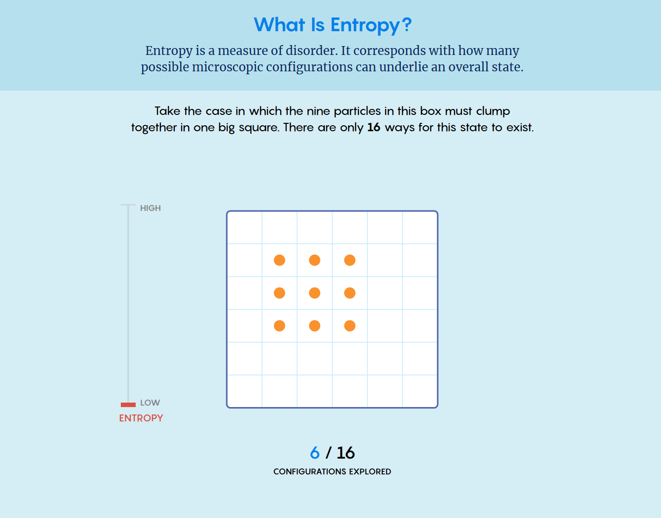
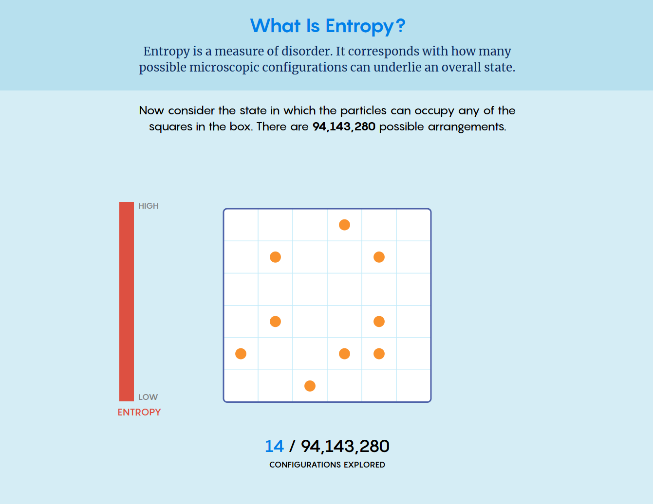
What Is Entropy?
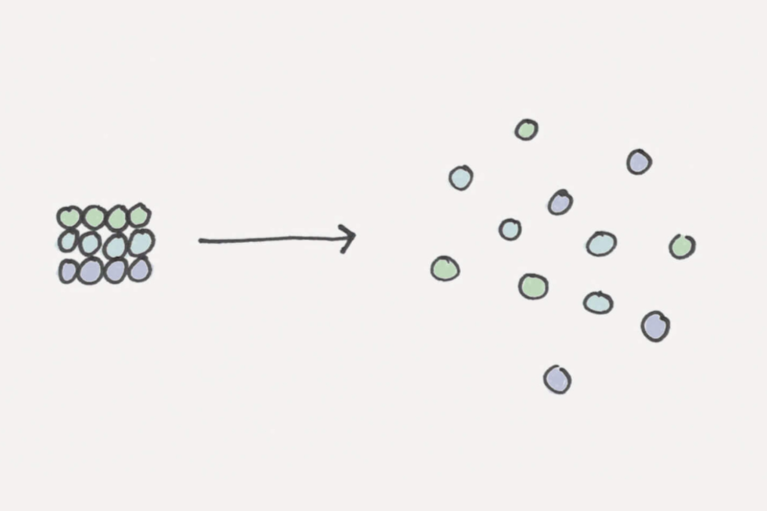
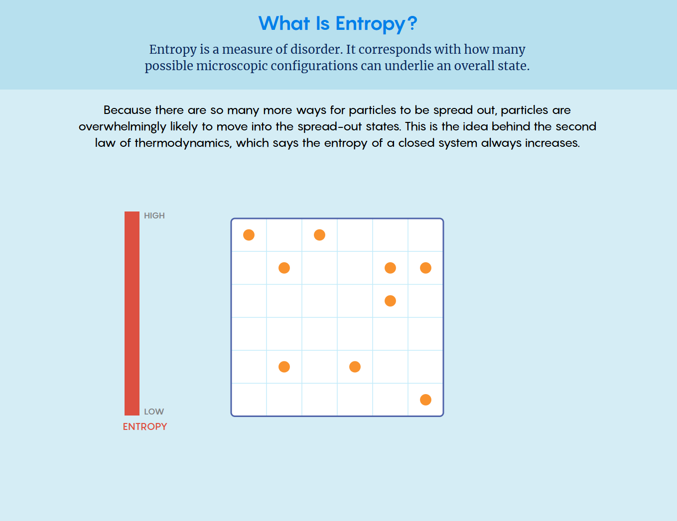
Imagine your bedroom right after you’ve cleaned it: your bed is made, your desk is organized, and your clothes are neatly put away. We can describe this as a low-entropy state because there are very few ways to arrange the room without creating disorder. In contrast, there are countless messy arrangements. Systems naturally tend to move toward these more disordered states simply because there are so many more! Entropy measures the amount of disorder or uncertainty in a system. More precisely, it counts the number of microscopic configurations (microstates) that correspond to the same overall condition (macrostate). Since disordered microstates vastly outnumber ordered ones, systems tend to evolve from low-entropy (ordered) to high-entropy (disordered) states.
Entropy Visualizations
Why Graphs?
Many real-world systems (epidemics, social networks, the internet, physical processes) exhibit entropy. Measuring that entropy helps us understand and predict their behavior. But these systems are too complex to model with continuous equations alone. By discretizing them and applying linear algebra techniques, we can study them more effectively. Graph theory provides a natural framework for this discretization: we represent complex systems as networks of vertices and edges and analyze their structure using matrices.
Types of Graphs
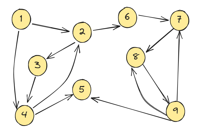
There are two main kinds of graphs: directed and undirected. In a directed graph, the edges have arrows showing the direction from one point to another, like in the image above. In an undirected graph, the edges don’t have arrows—they go both ways. In this research, we mostly look at undirected graphs, like the ones shown below.
- Path Graph: Vertices arranged in a line where each is connected to its immediate neighbors.
- Tree Graph: A connected graph with a unique path between any two vertices and no cylces.
- Cycle Graph: Vertices connected in a closed loop where each vertex has degree two.
- Star Graph: A central vertex connected to all others, which are otherwise unconnected.
- Lattice: A grid-like graph where vertices form a square, repeating arrangement.
- Torus: A lattice graph with edges wrapped around to form a donut-shaped topology.
- Complete Bipartite Graph: Vertices split into two sets with edges connecting every vertex in one set to every vertex in the other.
- Complete Graph: Every pair of vertices is connected by an edge.
- Types of Graphs Research Notes
Von Neumann Entropy
What Is Von Neumann Entropy?
Von Neumann entropy measures how complex or disordered a graph is by analyzing its structure. It is a measure of quantum information or uncertainty associated with a quantum state.
Read More about Von Neumann Entropy here
How We Calculate It
To compute the von Neumann entropy of a graph, we start by analyzing the eigenvalues (λ) of a special matrix called the Laplacian matrix (Δ). These eigenvalues capture important information about the graph’s structure.
The Laplacian matrix itself is calculated by combining two other matrices:
- Degree matrix (D): A diagonal matrix where each entry shows how many connections (edges) a vertex has.
- Adjacency matrix (A): A matrix that shows which vertices are directly connected. If two vertices share an edge, the corresponding entry is 1; otherwise, it is 0.
We form the Laplacian matrix by subtracting the adjacency matrix from the degree matrix:
\(Δ = D - A\)
Finally, the von Neumann entropy \(S\) is computed using the (non-zero) eigenvalues of the Laplacian as:
\(S = \sum \lambda \log \lambda\)
Example: Von Neumann Entropy of the Cycle Graph C₄
Step 1: Label vertices \(v_1\) through \(v_4\), connected in a cycle.
Step 2: Degree matrix \(D\):
\[
D = \begin{bmatrix}
2 & 0 & 0 & 0 \\
0 & 2 & 0 & 0 \\
0 & 0 & 2 & 0 \\
0 & 0 & 0 & 2
\end{bmatrix}
\]
Step 3: Adjacency matrix \(A\):
\[
A = \begin{bmatrix}
0 & 1 & 0 & 1 \\
1 & 0 & 1 & 0 \\
0 & 1 & 0 & 1 \\
1 & 0 & 1 & 0
\end{bmatrix}
\]
Step 4: Laplacian \(Δ = D - A\):
\[
Δ = \begin{bmatrix}
2 & -1 & 0 & -1 \\
-1 & 2 & -1 & 0 \\
0 & -1 & 2 & -1 \\
-1 & 0 & -1 & 2
\end{bmatrix}
\]
Step 5: Eigenvalues: \( \{0, 2, 4, 2\} \)
Step 6: Compute \(S = \sum \lambda \log \lambda\), excluding \(0\):
\[
S = 2 \log 2 + 2 \log 2 + 4 \log 4 \approx 8.3178
\]
Key Takeaways
- Entropy measures uncertainty: It tells us how unpredictable or disordered a system is.
- Entropy connects across many fields: It appears in thermodynamics, quantum mechanics, and information theory, where it helps explain how systems evolve, and how information is transferred or lost.
- Graphs help us model complex systems: By breaking systems into simpler, discrete parts, we can apply linear algebra techniques to study how they behave. Discretizing continuous systems into graphs makes them easier to analyze and helps us compute solutions more effectively.
- Von Neumann entropy brings these ideas together: It uses the eigenvalues of the Laplacian to quantify a graph’s entropy, providing insight into the network’s topology and complexity.